![]()
|
| Reinforcement
Learning -
|
About Reinforcement LearningReinforcement
learning is the process for a program to interact within an
environment and learn by receiving numerical rewards or punishment
while trying to obtain a goal. In this case, the goal is to win when
dealing with games. The environment is “where” and “how”
a program, that is using reinforcement learning, interacts against its
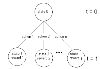
opponents in the game. A state
is represented by s, where s є S, and S is the set
of all possible states. The program, when playing the game, is in a
state and given a choice of options that are actions represented as,
a, where a є A, and A is the set of all possible
actions. Depending on the program’s decisions and actions, it will
make a transition from state st to state st+1.
The diagram below shows an example of a possible state-action tree.
The policy, π, is the set of rules, a function, or tables that maps actions, and/or states to the probabilities of a reward. The policy is what the agent uses to find the path to a reward without looking at each possible solution in the tree from the current state. The policy function is noted as πt(s, a), where at = a, if st = s. The policy influences the agent’s decision in implementing the game. Any subtle changes in the policy can change the way the agent explores or exploits the play of the game. Exploration is when an agent decides to explore the states and actions, not always taking the path to the best reward. Exploration allows for finding the majority of the paths if not all in which the best paths are found. A problem is that many games that are played will have to take up a large amount of memory or be played so often that it could take a large amount of time for the policy to be competitive. While in exploitation, the agent is encouraged to take the best path to the highest reward. This will allow for fewer games that need to be played, but it is necessary to explore and find possibilities. Exploration allows the agent to visit possible states that improve its outlook and allow for better game play. A use of both exploration and exploitation is necessary, where one alone will not be the best solution in developing learning. A combination of both or using a majority of exploitation and a little exploration is probably the best solution to finding competitive programs. These concepts are developed through a function that allows for the agent to see the predicted reward values; this function is called the value function. The agent follows a value function, which shows what the potential reward can be in the long run if the agent follows the current policy given by predicting the reward function. In any game, where players alternate moves, there is usually a set of sequences that can be grouped. This is called, in reinforcement learning, an episode. In an episode the last state is known as the terminal state. The majority of games are best modeled using episodes: the computer might make a play prompting its opponent to make a play thus, giving one episode. These set of episodes, in games, are given the name episodic tasks. The states without the terminal state will be noted as S and the states including the terminal state will be noted as S+. Now, let’s redefine reinforcement learning more clearly using the knowledge up to this point. Reinforcement Learning is a stochastic problem, where the value function may not represent the actual true value at first. This is due to estimation in the beginning and not every future event may be represented or known with certainty. By looking at what is expected, stochastic problems can be solved giving a solution that is optimal over a set of episodes. -=Evaluation Feedback
|
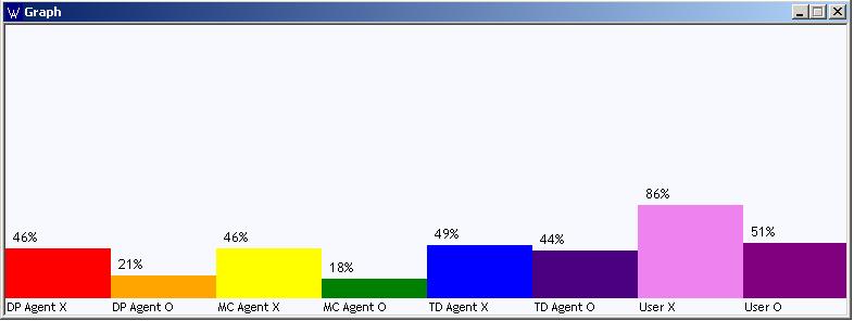
| Temporal Difference | Dynamic Programming | Monte Carlo | Exhaustive Search | |
| Learning | Raw | Model | Raw | None |
| Back Up Type | Sample | Full | Sample | Full |
| Back Up Depth | Shallow | Shallow | Deep | Deep |
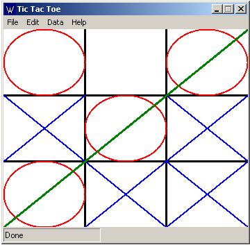
Microsoft Windows 2000/XP
Simply unzip the file and place the folder in the desire location. Run the [TicTacToe.exe] file to run the program.
To start playing a game, select File -> New -> Game and then select the type of game you want to play from Single Player vs. Computer, Two Player Game, or Simulation to have the computer play itself.
There are three different type of computer you can play against: Dynamic Programming, Monte Carlo, or Temporal Difference. The default is the Monte Carlo. To choose your opponent, go to Edit -> Opponent.
You can also change how the program learns for each of the computer
learning styles by going to
Edit -> Agent -> Learning Style -> [and select among the
three]
You can also change the amount of games the agent will play during simulation, I do warn not to make the value to large. I estimated that approximately 100 games is equivalent to 1 minute.
Under the Data in the menu items, you can view the results of win percentages, state values, the xml file, and total number of visited states so far.
[Andrus 04] Andrus, W., (2004). Reinforcement Learning in Games. Master’s Thesis, Presented to the Department of Computer Science at the State University of New York Institute of Technology in Utica, New York
[Bellman 62] Bellman, R., (1962). Dynamic Programming. Princeton University Press.
[Brafman & Tennenholtz 03] Brafman, R.I. and Tennenholtz, M. (2003). "Learning to Coordinate Efficiently: A Model-based Approach", Volume 19, pages 11-23. JAIR. Retrieved June 25, 2004 from http://www-2.cs.cmu.edu/afs/cs/project/jair/pub/volume19/brafman03b.pdf
[Conitzer & Sandholm 04]Conitzer, V., Sandholm, T., (2004). Communication Complexity as a Lower Bound for Learning in Games. In Proceedings of the 21st International Conference on Machine Learning (ICML-04), Banff, Alberta, Canada. Retrieved June 24,2004 from http://www-2.cs.cmu.edu/~conitzer/conitzer_sandholm_comm_games.pdf
[Conitzer & Sandholm 03] Conitzer, V., Sandholm T., (2003). BL-WoLF: A Framework For Loss-Bounded Learnability In Zero-Sum Games. In Proceedings of the 20th International Conference on Machine Learning (ICML-03), pp. 91-98, Washington, DC, USA, Retrieved June 24, 2004 from http://www-2.cs.cmu.edu/~conitzer/conitzer_sandholm_blwolf.pdf
[Meyer 98] Meyer, F., (1998). Java Black Jack and Reinforcement Learning. Logic Systems Laboratory, EPFL. Retrieved July 20, 2004, from Swiss Federal Institute of Technology-Lausanne, Switzerland. http://lslwww.epfl.ch/~aperez/BlackJack/classes/RLJavaBJ.html.
[Mitchell 97] Mitchell, T., (1997). Machine Learning. MIT Press, Singapore.
[Nilsson 98] Nilsson, N., (1998). Artificial Intelligence: a new synthesis. Morgan Kaufmann Publishers, Inc., San Francisco, California.
[Schaeffer & van den Herik 01] Schaeffer, J., and van den Herik, J., (2001). Games, computers, and artificial intelligence. Elsevier Science B. V.
[Sutton & Barto 98] Sutton, R. S., and Barto, A. G. (1998). Reinforcement learning an introduction. MIT Press, Cambridge, MA.
[Tesauro 95] Tesauro, G., (1995). Temporal Difference Learning and TD-Gammon.Communications of the ACM 38, 58-68.
 An agent is what decides, in the program, the paths to take
when given a state and/or actions to maximize the rewards it could
receive. The maximization of rewards is defined as the expected
return, Rt = rt+1 + rt+2 + …+ rT
where T is the last time step. The agent has no control over the
environment and the rewards it receives. The agent may have knowledge
of everything in the environment or it can be limited. As in the case
of card games, the agent should not have the ability to see what the
other players are holding. The agent follows a policy that will help
it find a path, giving high rewards.
An agent is what decides, in the program, the paths to take
when given a state and/or actions to maximize the rewards it could
receive. The maximization of rewards is defined as the expected
return, Rt = rt+1 + rt+2 + …+ rT
where T is the last time step. The agent has no control over the
environment and the rewards it receives. The agent may have knowledge
of everything in the environment or it can be limited. As in the case
of card games, the agent should not have the ability to see what the
other players are holding. The agent follows a policy that will help
it find a path, giving high rewards.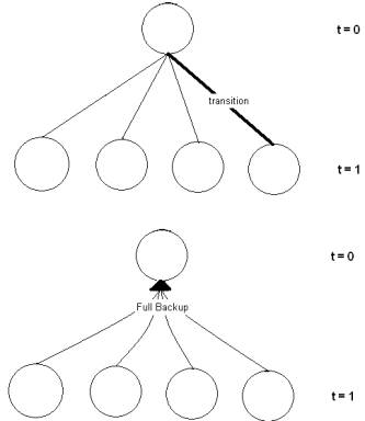 Now
skipping ahead... Dynamic Programming is one of the many techniques used in
Reinforcement Learning for evaluating the value of an state. In Dynamic
Programming the values of each successor state of st are backed up
together by the value function; this is called a full backup. All backing up in
dynamic programming is done this way. The agent first selects the best value
given the policy, when this is done, the back up process begins for that state.
Of all the possible state's values that could have been reached are used to
update the previous seen state. The process of backing up is done after each
move.
Now
skipping ahead... Dynamic Programming is one of the many techniques used in
Reinforcement Learning for evaluating the value of an state. In Dynamic
Programming the values of each successor state of st are backed up
together by the value function; this is called a full backup. All backing up in
dynamic programming is done this way. The agent first selects the best value
given the policy, when this is done, the back up process begins for that state.
Of all the possible state's values that could have been reached are used to
update the previous seen state. The process of backing up is done after each
move.